Black Planet Ratio

The Paris Agreement of Dec. 2015

Several posts in Open Mind argue that the Paris Accord goals are unsatisfactory. For one, there is too much uncertainty in the pre industrial global temperature to use it as a basis. A better basis would be the best estimate of global temperature from a well characterized recent time frame such in 2015, the year of the Paris Agreement, or 1951 to 1980. Another problem, however, is that global temperature is affected by the sun. Humans have no control of the sun. A better climate metric would imply something over which humans have an influence.

This post explores alternate metrics, all based on comparing the earth, a very complicated planet, to a simple, hypothetical planet with the same rotation and orbit as earth, but with no atmosphere and with a black surface.

The reason to compare earth to a black planet is that the temperature of a black planet and its radiation energy budget can be easily calculated. If a black planet had a global temperature, T_BP, then the energy it would be radiating per unit area and unit time ( radiant exitance) would be given by the Sefan-Boltzmann Law.

where σ is the Stefan-Boltzmann constant and ETR is the magnitude of the emitted thermal radiation. The temperature, T, is in units of absolute temperature. A black planet would absorb all incoming solar energy. At equilibrium the ETR of a black planet would be equal to the incoming solar flux, IN. The equilibrium temperature of a black planet would be given by

Earth’s mean global temperature is complicated. It depends on the incoming solar flux and on conditions on earth that can be affected by human activity. I define the black planet ratio, BPR, as

Note that this definition of BPR depends on how global temperature is measured or defined. Here I will use the global mean surface air temperature at a height of 2 meters.

Conditions on Earth

The earth is not black. Plus, it has an atmosphere with clouds, aerosols, and a greenhouse effect. Since the year 2000 NASA has been using the CERES satellite and other instrument systems that “precisely track changes in Earth’s radiation budget with remarkable precision and accuracy.” CERES publishes the following parameters:

IN = Incoming solar flux

ETR = Emitted Thermal Radiation, Top of the atmosphere long wave flux – all sky

ASR = Absorbed Solar Radiation, (Incoming Solar flux) minus (Top of the atmosphere short wave flux – all sky)

Note two radiations emanating from earth. The radiation emanating from earth is not just heat radiation. The earth also reflects, i.e. does not absorb, nearly one third of the incoming solar radiation. The CERES scientists can separate the two components because reflected solar radiation has a much higher energy or shorter wave length than does the heat radiation. The absorbed solar radiation, ASR, equals the incoming flux minus the reflected short-wave flux. The earth’s reflectivity or albedo, α, can be defined by the following relation

The reflectivity of the earth depends on what is on the surface. Ice and snow are more reflective than water or forest. It also depends on what is in the atmosphere. Clouds and aerosols are more reflective than clear sky.

The much longer wave radiation, ETR, is the emitted flux due to the earth’s heat. Just as for a black planet, it is proportional to the fourth power of global mean surface temperature, but the proportionality constant is less than the Stefan-Boltzmann constant. As shown below, the ratio of the earth’s ETR to that of a hypothetical black planet at the same temperature can be used to estimate how hot the earth will get, if all current conditions, including ASR, remain the same. In other words that ratio, ε, call it the earth’s effective emissivity, can be used to estimate the earth’s temperature set point.

The following shows ASR and ETR since 2000. (See Earth’s Energy Imbalance Chart in Global Temperature Report for 2023 posted by Robert Rohde.)

At equilibrium the emitted thermal radiation, ETR, will equal the absorbed solar radiation, ASR. If the emissivity ratio remains the same, then

or, simplifying,

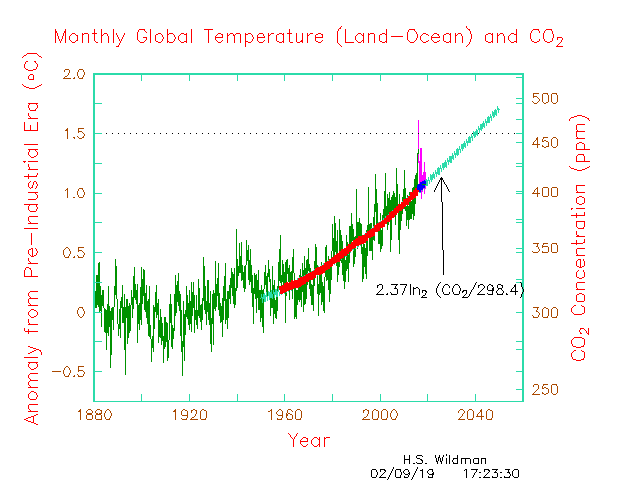
This is a powerful result because it directly shows that if the earth is in energy balance (emitted flux equals absorbed flux), the equilibrium temperature is equal to the current temperature. When the absorbed flux is greater than the emitted flux, the equilibrium temperature must be higher, and the earth will warm. The equilibrium temperature is where the earth is headed, but it is not necessarily the final temperature. There are feedback processes that could change the set point, either amplifying or counteracting the warming. Changes in earth’s energy budget – whether from increased greenhouse gases, changes in albedo, or other factors – will lead to changes in global temperature. The following graph shows how the equilibrium temperature has compared to global temperature since the year 2000. For global temperature I used the 2-meter surface temperature estimates of ECMWF Reanalysis version 5 (ERA5) from the Climate Reanalyzer web site. The global temperature and the CERES earth energy parameters have large seasonal dependencies. One way to avoid the large swings is to only plot yearly averages. Another method, one used by Robert Rhode, is to plot the one year moving average. Here is the 1 year moving average of global temperature from 1940 and the equilibrium temperature from 2000 to the present. There is a range of suggested values for preindustrial temperature. One, for example, is 0.87°C less than the average global temperature between 2006 and 2015. For this I calculate it as 286.7°K.

Equilibrium Temperature

Note that in the year 2000 the equilibrium temperature was only slightly higher than global temperature. Even though the planet was warming, it was close to being in equilibrium. Since then, the gap between the current temperature and equilibrium temperature has gradually increased by about 0.15°C per decade until in 2024 the gap is about 0.4°C. The earth cannot keep up with the rapidity of the changes. It is analogous to cooking a turkey. When the set point of the oven is increased quickly the temperature of the turkey goes up, but how fast it goes up depends on the size of the turkey. The equilibrium temperature is like the oven set point. The earth’s climate system is a very big turkey. It has a large heat capacitance, so it takes time. The graph shows that global temperature now is close to 1.5°C above preindustrial levels. The equilibrium temperature, however, has exceeded the 1.5°C goal since 2016. Just one year after the Paris Agreement the earth’s set point exceeded the goal.

Comparing the equilibrium temperature with the previously defined Black Planet temperature, one gets

or, substituting the definitions for ε and α,

In summary

And

Arguably, BPR_eq is a better metric for a climate accord than global temperature. It only depends on conditions on earth and directly indicates what factors need to be controlled to “set” the global temperature that will meet our goals. The following graph shows BPR since 1941 and BPR_eqsince 2000. Again, all values are one year moving averages.

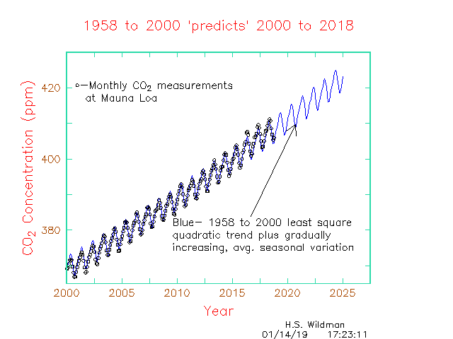
Also shown in the graph is how BPR correlates (very well) with atmospheric CO_2.. This is essentially the same information as the first graph except that now it indicates the two controlling parameters, namely α and ε. BPR_eq is the earth’s set point. When the incoming solar flux, IN, is factored in, BPR_eq gives the earth’s set point.

Assuming an average value for IN, BPR_eqis well above the 1.5°C goal. Given current conditions, it is inevitable that 1.5°C will soon be exceeded.

It’s interesting to see by how much BPR_eq and the individual parameters which contribute to it have changed since 2000. The next graph shows BPR_eq, (1-α), and (1/ε) relative to their values in 2000.

The (1/ε) factor is a measure of the greenhouse effect. Since 2000 it has increased by 0.531%. The (1-α) factor is a measure of how much of the incoming solar energy is absorbed. In the same period, it has increased by 0.791%. The combined effect, namely BPR_eq , has increased by 1.33%. At least since 2000, the amount of heat being absorbed, the (1-α) factor, has been increasing faster than the amount of heat being retained by the extra greenhouse effect, the (1/ε) factor. The earth is reflecting less radiation. This could be due to less ice coverage or to fewer aerosols. Some causes are discussed in this reference by J. Hansen, et. al. Uh-Oh. Now What?

Seasonal Variation

In the previous graphs the seasonal variation was suppressed by plotting the 12-month running average. All the previous parameters, namely T, BPR, α, and ε show large seasonal variations. Climate scientists worry about a 1.5°C to 2°C change in global temperature from the beginning of the industrial period in 1760. Yet the 2-meter global air temperature varies by about 4°C every year from a minimum in mid-January to a maximum at the end of July! That is a huge change!

Here is the 2-meter global air temperature for 2024.

Why does mean global temperature peak in the summer? The next graph compares the seasonal variation of the 2-meter global temperature, T, to the forth power with the incoming solar flux, IN. The earth’s orbit is an ellipse with a small eccentricity of about 0.0167. Incoming solar should be at a minimum when the earth is farthest from the sun, which is about July 5.

Incoming solar precisely follows the inverse square of the distance to the sun. One would think that global temperature would follow the seasonal dependence of the solar flux. It shows the opposite trend. Global temperature peaks when the earth is farthest from the sun. The seasonal variation of α and ε may help explain why. The following graph shows that variation.

The reflectivity or albedo, α, has a strong seasonal dependence with two peaks, the larger peak in December and January, the smaller peak in April and May. The emissivity factor, ε, has a smaller seasonal variation. Higher reflectivity means cooler temperature. Lower reflectivity means hotter temperature. This makes sense. In January the earth is tilted to expose more of reflective snow of Antarctica to the sun. In June Antarctica is tilted away. See two images of the earth from the DSCOVR satellite below. The first is from Jan. 15. The second is from June 28. By eye, the first image has higher average brightness. The southern hemisphere, which is tilted toward the sun in January, has more ocean. More ocean may mean more clouds.

In conclusion, I estimate that we reached a “setpoint” temperature of 1.5°C above preindustrial in 2018. We are well on our way to reaching a “setpoint,” i.e. a point of no return, of 2.0°C by 2032.

Effect of the Covid-19 Pandemic on Atm. CO2

NOAA asserts that, although the Covid-19 pandemic has led to clearer skies and fewer fossil fuel emissions, the effect on rising CO₂ in the atmosphere will be negligible. This could be verified by looking for a deviation from the current trend. There is no physics in a trend line, but, if the trend is sufficiently consistent, it could be reasonably be used to measure the magnitude of an effect.

The trend in the season corrected concentration of CO₂ looks to be very consistent. Below is the 62-year record of measurements from Mauna Loa, also known as the Keeling Curve, shown together with a 3-parameter trend line. In 1958 the slope of the trend line is 0.865 ppm/year. By Jan. 2020 it is 2.47 ppm/year. The concentration of CO₂in the atmosphere is increasing at an accelerating rate. Month to month the slope of the trend line agrees with the actual slope to within a std. deviation of 0.6 ppm/year.

The seasonal variation also looks to be consistent. Here it is after subtracting the season corrected concentration.

One way to determine its shape is to average the seasonal variation over the 62 years. Instead I’ll use a matrix technique called Principal Component Analysis (PCA). The first principle component is the unique seasonal variation or shape that accounts for the most variance over 12 months. The technique also determines a magnitude of that shape for each of the 62 years. The second principle component is the unique seasonal variation or shape that accounts for the most variance after the first component is subtracted from each year’s variation. And so on for 12 unique shapes. It’s easier to show the result than to explain it. In this case two components accounted for 99.94% of the data. The other components are increasingly irregular, more like noise. Here are the two components. The shapes of seasonal variation are on the left. The magnitude of the corresponding shapes for each year are plotted on the right.

The first component accounted for 99.62% of the data. Although the magnitude varies, the shape of the seasonal variation has remained very consistent. The magnitude of the main seasonal variation increased by 22% from 1958 to 2020. Maybe the size of the variation is proportional to the concentration of already in the atmosphere. There are also year to year differences in the magnitude, with maxima in 1966, 1979, 1994, and 2016, and minima in 1970, 1987, 2000, and 2010. Maybe varying patterns of precipitation and drought in the Northern Hemisphere cause these changes in magnitude. The second component only accounts for 0.32% of the data, but I kept it for the model trend because it did not look like noise. It represented a slight change in the shape of the seasonal variation with time. The size of this change also seemed to change linearly with .

To model the trend in seasonal change, I used the two component shapes plus least squares fits of the magnitudes with atmospheric CO₂. This is just a reasonable, but unproven assumption, I could have used years as the independent variable. Below in animated gif is a comparison of the raw seasonal variation, the two-component reproduction from PCA, and the constructed trend model in seasonal variation. The 2-component model gives a smoothed near perfect fit to within a std. dev. of 0.061 ppm. (Of course, a 12-component reconstruction gives a perfect fit.) The fit of the constructed trend is only slightly worse to within a std. dev. of 0.094 ppm.

The final season corrected trend model is compared with the 62-year Mauna Loa record of atmospheric CO₂ below. The fit is to within a std. deviation of 0.74 ppm.

That’s a consistent, increasing, 62-year trend line. I’ll compare future measurements of CO₂ to this trend to monitor the effects of human actions either in reaction to Covid-19 or to climate change.

After realigning the trend line for the atm. CO₂ value at the beginning of 2020, the trend along with 3 sigma (standard deviation) lines is shown for the next three years. Also plotted are individual Mauna Loa measurements of CO₂. In the first 4 months of 2020 no difference from the trend is detected.

This result is discouraging to the goal of slowing the rate at which CO₂ is increasing, much less stopping the increase, by individual actions such as reducing travel.

A Problem with Trends

What is clear is that there has been no change in either greenhouse gas or global temperature trends since the Paris Agreement on Dec. 15, 2015. There has been no progress and there is none in sight. Given current trends, the question then is, when will global temperature reach the agreed upon 1.5°C limit. For this question a post at Tamino’s Open Mind blog is informative. He calculates that at 435 ppm CO2 in the atmosphere in about 2029 the earth would have reached it’s “carbon budget” for avoiding the 1.5°C limit. But estimates for the remaining “carbon budget” vary. Some uncertainty is due to vague definition. The reference period for the 1.5°C limit is poorly defined. There is disagreement on whether to use atmosphere or surface temperature. It was pointed out in discussion that other greenhouse gases should be included in the “budget” calculation. A reference was given to a NOAA/ESRL published graph showing how the mixture of all greenhouse gases have varied with time in units of the equivalent concentration of CO2 in ppm. There is also the question whether to allow for climate inertia, the lag time in temperature. It’s analogous to putting a roast in the oven. The oven heats the meat, but it takes time for the center of the roast to reach the right temperature for rare, medium, or well done. By reducing the heat energy radiated into space, greenhouse gases change the earth’s energy balance, but it takes time to heat the rocks, warm the oceans, and melt the ice. Maybe a better analogy is a bus traveling at 75mph. When will slamming on the brakes prevent it from going over the cliff and when would it otherwise go over the cliff?

I wondered what the no-lag time for reaching 1.5°C would be if current trends continue. For temperature I chose the NASA and Berkeley (first table) temperature records. Following the publication by Ed Hawkins, et. al., I referenced the period between 1986 and 2005 as being 0.68°C above the preindustrial period, referenced as the global temperature between 1765 and 1800. I used either the CO2 Keeling curve from NOAA or the “CO2 equivalent” for all greenhouse gases from NOAA/ESRL for fitting to global temperature.

I found that “trends” can lead to two different answers. As Tamino’s graph showed, the pattern of CO2 over the past 60 years has been very consistent. For this entire period global temperature can be fit within a standard deviation of 0.16°C to 2.5 times the base 2 logarithm of the concentration of CO2 in ppm divided by 301.2. If this relation and trend continue then we could expect to reach the 1.5°C limit by 2039 with 456 ppm CO2 in the atmosphere. However, that was ignoring all of the other greenhouse gases. The pattern or trend for the CO2 equivalent of all greenhouse gases combined has not been as consistent, but global temperature for the past 60 years can also be fit within a standard deviation of 0.16°C to 1.6 times the base 2 logarithm of the ppm CO2 equivalent for all greenhouse gases divided by 319.4. Extending this relationship and trend reaches the 1.5°C limit in 2062 with a 612 ppm CO2 equivalent mixing ratio of all greenhouse gases.

Here is the analysis.

CO2 data is surprisingly predictive. There’s a seasonal variation, which can be understood from the distribution of vegetation covered land on the planet, but the seasonal variation is superimposed on a near perfect quadratic. To model the trend, I used a least square fit of the 1958-2000 monthly data to a second order polynomial, i.e. a quadratic curve. For the seasonal variation I averaged the difference from the quadratic for each month. I also noticed and included that the magnitude of the seasonal trend gradually increased, maybe because it depends on the amount of in CO2 the atmosphere. The CO2 data and the trend are plotted below. Plotted with it is the CO2 equivalent and straight-line trend for all greenhouse gases over the same period. I estimated the points from the NOAA/ESRL graph. (Neither curve shows any tendency to a downward change after the Paris Agreement in 2015.)

The following graph compares the 225 monthly measurements at Mauna Loa since the year 2000 with the “predictions” from the model trend based on the 502 monthly measurements from 1958 to 2000. The 1958 to 2000 model “predicts” the measurements since the year 2000 to within 1 ppm.

There certainly is no sign that the trend in either CO2 or the CO2 equivalent of all the greenhouse gases has changed since the Paris Agreement in December 2015.

The next question is how this ever-increasing level of greenhouse gas will affect global temperature. Here is a graph showing the least squares fit of temperature to the log of CO2 for the past 60 years. As shown below, the fit is so good that one is tempted to extrapolate this relation to future years using the current trend of CO2.

This fit neglects, however, that the other non-aqueous greenhouse gases affect temperature. It’s probably more correct to instead use the CO2 equivalent for all greenhouse gases. Since I couldn’t find a table with the CO2 equivalent ppm values dating back to 1958, I estimated them from the graph. Below is the resulting analysis. For the previous 60 years the fit is just as good, but including other greenhouse gases bends the future trend downward.

For 60 years the trend in global temperature can also be very well fit to either the logarithm of just CO2, ignoring the other greenhouse gases, or the logarithm of the “CO2 equivalent” of all greenhouse gases in the atmosphere. Including other greenhouse gases changes the trajectory of the trend for future years. Using just CO2 predicts reaching the cliff in 2039 with 456ppm CO2. Using the CO2 equivalent for all greenhouse gases predicts reaching the cliff in 2062 with a CO2 equivalent of 612ppm or when CO2 concentration would be 530ppm.

In summary, for a cliff at 1.5°C, Tamino’s analysis suggests slamming on the brakes in 2029 at 435ppm CO2. My analysis looked at two trends, one for CO2 and one for the CO2 equivalent of all gases. The CO2 trend and fit to global temperature predicts the cliff in 2049 at 456ppm. The CO2 equivalent trend for all greenhouse gases predicts the cliff in 2062 at a CO2 equivalent 612ppm or a CO2 concentration of 530ppm. Using the Berkeley record showed similar results using CO2 or CO2 equivalent. Tamino’s result may be the best current estimate. Mine, based on trends, are not far removed. Prudence would dictate a moon shot size effort to eliminate human emissions of greenhouse gases.

I will be looking for a change in the trajectory for when measurements of CO2 and global temperature show actual progress in our goal to avoid the 1.5°C cliff.

Climate Sensitivity

I’m trying to understand the climate sensitivity. To me it is too vague a concept. It is the increase or decrease in global surface temperature due to a given climate forcing. By convention, the given climate forcing is equated to that of a doubling of the concentration of CO₂ in the atmosphere. Apparently, climate sensitivity includes all feedbacks. Its ok that it includes a humidity feedback, i.e. the feedback which arises because the solubility of water in air and the evaporation rate of water are temperature dependent. It also includes cloud feedbacks. Apparently, though, it includes feedbacks that may take a really long time or feedbacks that may vary due to other conditions. For example, ice sheets take a long time to melt away. Also, the vulnerability of ice sheets change depending the current global temperature. Some feedbacks change the average reflectivity, the albedo, of the earth. Some affect the earth’s emissivity. I would be satisfied to know the response of the earth’s emissivity to a doubling of the concentration atmospheric CO₂. For small changes, that’s equivalent to knowing the value of “B” in the following equation.

Where x is the base 2 log of CO₂ concentration.

The current value of earth’s emissivity is defined by applying the Stefan-Boltzmann equation to the earth. At equilibrium the radiation from the earth must balance the radiation received from the sun.

T is earth’s average surface temperature. Epsilon is the earth’s average emissivity. Sigma is the Stefan-Boltzmann constant. TSI is the total solar irradiance at the position of the earth. The solar irradiance is intercepted on a disk the size of the earth, but, since the earth spins, it is absorbed over a sphere. The area ratio of the disk to the sphere is ¼. Alpha, the albedo, is the fraction of incoming radiation that is simply reflected back into space. Solving for epsilon gives the following equation for emissivity.

Satellites measure the current value of alpha at about 0.3. The current value of TSI is about 1361 W/m₂ . Current average global temperature is about 287°K. Therefore, from the above equation the current value of emissivity is about 0.619. Solving the above equation for T gives

If we knew the value of “B” we could the obtain the (partial?) climate sensitivity by taking the partial derivative of T with respect to x, the base 2 log of CO2.

Or substituting the above values

So, the partial climate sensitivity due to the effect of CO₂ on emissivity is 116 times “B”. The previous equations can be used to calculate emissivity knowing solar irradiance, average global temperature, and albedo. Although there are good records of irradiance and global temperature, I haven’t found good records or even good estimates of albedo. Albedo could vary for a number of reasons, such as ice sheet extent, black carbon on snow, cloudiness response, and aerosols from volcanoes and human emissions. The longest record I found was satellite measurements from 2000 to 2011. During that period, it remained relatively constant at about 0.3. The following graph shows calculated emissivity, assuming albedo has remained constant, plotted versus the base 2 logarithm of atmospheric CO₂. Since 1958 the levels of CO₂ in the atmosphere have been very precisely measured, so only data from 1958 to 2019 is plotted.

The result is a straight line with scatter. The correlation coefficient between the calculated emissivity and the log of CO₂ is 0.9. A least square fit gives “B”, i.e. the slope, a value of 0.021. Multiplying by 116 gives an estimate of 2.44 to the (partial?) climate sensitivity with the assumption that albedo stayed constant at 0.3.

A value of 2.44 for the climate sensitivity is surprisingly close to 2.36, the 1967 result for CO₂between 300 and 600ppm, fixed relative humidity, and average cloudiness in S. Manabe and R. T. Wetherald. That paper assumed that relative humidity would remain constant with small increases in atmospheric temperature. Since water solubility in air increases with an increase in temperature, absolute humidity increases if relative humidity remains the same. Manabe/Wetherald computed eight values for the climate sensitivity to atmospheric CO₂. Four conditions were fixing absolute humidity, fixing relative humidity, having average cloudiness, and having clear skies. Two ranges in CO₂ were 300 to 500ppm and 300 to 600 ppm. I’ll focus on the 300 to 600 ppm values. In the case of absolute humidity remaining constant the chemical sensitivity was 1.33 for average cloudiness and 1.36 for clear skies. In the more likely case of relative humidity remaining constant the chemical sensitivity was 2.36 for average cloudiness and 2.92 for clear skies. The above 2.44 result derived from the NASA temperature record is in remarkable agreement with the Manabe/Wetherald value of chemical sensitivity for average cloudiness. This agreement could be luck. Average albedo could have changed between 1958 and now. Also there are other greenhouse gases other than CO₂. The proper way to determine climate sensitivity is include all the variables in realistic models. I did this exercise as a sanity check. The result was within the margins of sanity.

It is unsatisfactory, however, that I did not include other greenhouse gases, since they contribute to the climate forcing of the greenhouse effect. Including them would logically reduce the above climate sensitivity. Fortunately, NOAA has estimated an equivalent CO₂ concentration for all greenhouse gases for the period from 1700 to present. They didn’t show the numerical data, but I estimated it from their graph. Below is a comparison of CO₂ concentration and CO2 equivalent concentration from NOAA/ESRL.

Using my estimate of CO₂ equivalent from the NOAA/ESRL graph, I calculated emissivity for the 1958 to present time period again assuming an albedo of 0.3 for that time period. This time I included both the NASA and the Berkeley global temperature records. Here is the result after plotting the values versus the logarithm to base 2 of CO₂ equivalent concentration.

The result was a straight line with scatter. The correlation coefficient was 0.875. From a least square fit of the data, this time, the slope “B” was determined as 0.0138. Again, multiplying by 116 gives a climate sensitivity of (116×0.0138) of 1.6°C. It again meets the sanity check. This value is less than the Manabe/Wetherald result for constant relative humidity and average cloudiness, but it is higher than their result for constant absolute humidity and clear skies. It also falls within the likely range of 1.5°C to 4.5°C stated in the IPCC Fifth Assessment report.

Albedo, what would it have to be (again)?

As before I’m interested in “natural” internal cycles that cause global temperature to oscillate or vary around an equilibrium temperature. In a previous post I used the Berkeley temperature record. This time, with slight changes in method, I’m using the discrete Fourier transform, DFT, on the NASA temperature record instead of the Berkeley record to find the periods of cycles required to reconstruct the record. First, I need to subtract out the equilibrium temperature. A problem is that the equilibrium temperature also varies and I have no record of what it should be. Another is that some ocean cycles may have very long periods, too long to be deduced from the modern temperature record. I can try to estimate equilibrium temperature. Aside from very minor contributions from the earth’s interior and from the rest of the universe, earth’s equilibrium surface temperature depends on only three factors, solar irradiance, albedo, and emissivity. There is a reasonably good record for solar irradiance, but not for albedo and emissivity. Furthermore, these two factors, albedo and emissivity, are internal to the earth and are affected by natural “internal” cycles, i.e ocean cycles. One approach would be to assume that most of the variations are due to natural cycles and to perform the DFT directly on the temperature record after subtracting the average, or the straight-line trend, or the long-term smoothed trend. Since my main interest is in ocean cycles, I want to eliminate factors, such as human induced changes to greenhouse gases, that are not part of natural cycles. I’ll assume that emissivity is a log function of atmospheric CO2 and that albedo has stayed relatively constant during the past 60 years and does not depend on CO2. The estimates and assumptions here are just hypotheses. In other words, “if I assume these values for albedo and emissivity, then these must be the ocean cycles.”

The best estimate for albedo in recent years is 0.3, i.e. about 30% of the sun’s energy is reflected back into space. Satellite measurements have found no consistent trend in albedo, at least in the years 2000 to 2011. To begin this fanciful exercise (If we assume this, then this must be true.), I assume an albedo of 0.3 for the entire Keeling time period, 1958 to now. I then use solar irradiance and the NASA temperature record to calculate emissivity. Below is the calculated emissivity plotted and fitted versus the log of CO2. As expected, the result is a straight line correlation. The plot below is for the entire temperature record since 1880. The correlation coefficient for the entire period is a negative 0.8869. For just the Keeling period from 1958 to now it is a negative 0.9. The fit below is for the Keeling period.

If this a reasonable fit of emissivity versus atmospheric CO2, I can then solve for what the albedo would have to be to account for the residual variance in global temperature. The result is shown below.

The average is 0.29957 with a standard deviation of 0.53%. It’s surprising to me that such a small variation in albedo could account for all the residual variance in global temperature after accounting for solar irradiance and the greenhouse effect. Replotting the same data on a compressed scale emphasizes this point.

Now with values for albedo, emissivity, and solar irradiance I could reconstruct the global temperature exactly. Instead I’ll use a 30-year smooth (Satitsky-Golay) of each factor to construct a trend line.

Here are percent changes of the three factors in the trend line model.

The factors based on albedo and emissivity show the highest percent change. Surprisingly (to me), the TSI based factor was constant to within 0.004%. As expected, the albedo-based factor was relatively constant from 1958 to present. Before 1958 it varies up to 0.1%. The emissivity based factor varies the most from about -0.1% to about 0.3%.

The next graph shows the NASA temperature record with the newly calculated trend line.

Below is the residual from the 3-factor trend line.

By the same method here is the residual from the Berkeley temperature.

Here is the Berkeley record with trend line.

In both the Berkeley and NASA record the strongest cycle was the one with yearly periodicity. After that the two records differed. For the Berkeley record the next 4 strongest cycles were those with periodicities of 5.82, 3.59, 9.93, and 4,56 years. For the NASA record the next four strongest cycles had periods of 6.04, 4.63, 3.56, and 8.68 years. I had expected closer agreement. Maybe together the 6.04- and 4.63-year cycles in the NASA record correspond to the 5.82 year cycle in the Berkeley record. The 3.56-year NASA and 3.59-year Berkeley cycles are identical. The comparison below shows that the 4 cycle reconstructions show only rough correspondence.

The graph below shows the NASA 3 factor trend line together with the Berkeley temperature record and trend line.

Comparing calculated albedo from Berkeley and NASA temperature records.

The graph below shows the calculated albedo from the Berkeley and NASA temperature records.

The method used to calculate albedo was strictly hypothetical, so now the obvious question is how did the average earth albedo vary from 1850 to 2019? Changes in albedo can derive from many different causes, such as ice sheet coverage, black carbon or soot on snow, vegetation changes, and aerosols in the atmosphere from volcanoes or human emissions. Competing causes could cause a oscillating changes in albedo. Another possibility is that albedo has remained constant and that the above variations are due to ocean cycles.

A bet on global temperature for 2019

Although it’s an anticlimax because he conceded months ago, my bet with a friend is now complete because NASA, back to work after the government shutdown, has reported the temperatures for December. My friend has already paid up with a beer after golf.

Here is a recap. My friend predicted that 2018 would not be in the top five hottest years, in other words, 2018 would have lower average temperatures than 2010. I bet that he was wrong. The final result (NASA temperature record) is that 2018 was 0.13°C hotter than 2010 and 0.02°C hotter than my precise prediction.

He’s currently admitting to recent warming, but not human’s responsibility. I’m trying to get him to make a new bet. (I really enjoyed that beer!) My proposed bet is that 2019 will also be hotter than 2010.

My exact prediction is that global temperature will average 0.13°C (+/- 0.164°C) hotter than 2010. I’m giving up a lot saying just hotter than 2010.

Here is how I make the prediction.
I found that monthly CO2 measurements are following a very predictable pattern that I modeled with a quadratic fit to the yearly data between 1958 to 2000 plus an average seasonal variation by month.

It’s amazing to me how closely the monthly values since the year 2000 have been following this model, month to month and year to year.

It’s also amazing that global temperatures are closely following atmospheric CO2. In a 1966 a paperS. Manabe and R.T. Wetherald made the very simple assumption that relative humidity would remain constant to calculate that between 300ppm and 600ppm of CO2 in the atmosphere global temperature would increase by 2.36 times the base 2 logarithm of CO2. My fit to the NASA temperature data found the multiplier to be 2.37! I don’t think this is a coincidence.

The following, kind of busy graph, shows the data for 2018 and my prediction for 2019.

Essentially my bet is that both CO2 and global temperature will remain within a little less than one standard deviation of a model based on the very narrow assumption that global temperature is going up only because of human emissions of CO2 (and assuming humans will continue to increase emissions). I’ll edit this post if my friend accepts the bet.

Albedo, what would it have to be?

Natural cycles

I’m interested in “natural cycles” or “natural variability” in the global temperature record. A cycle implies that there is a regular oscillation around an underlying equilibrium. Before I try looking for regular cycles I’d like to understand and subtract out where equilibrium temperature should be.

Usually the climate scientists estimate climate forcing’s to model equilibrium temperature. (https://data.giss.nasa.gov/modelforce/) I wanted to explore a different way, using just solar irradiance, greenhouse gases, and earth’s albedo. I should have used published values for climate forcing’s because they include all greenhouse gases, but couldn’t in my brief search find tabulated data, so here I use only values for CO2.

Three-Factor modeled trend line

Despite all the complexities, in the long run, there are only three factors that determine the equilibrium surface temperature of the earth. One factor, of course, is the radiant energy received from the sun. The radiant energy (flux) per unit area at the orbital position of the earth is called the total solar irradiance (TSI). Here is a reconstruction of TSI by G. Kopp and others. https://spot.colorado.edu/~koppg/TSI/TIM_TSI_Reconstruction.txt

The earth intercepts the TSI flux with the area of a disk the size of the earth. The earth rotates so this energy is distributed over the spherical surface area of the earth, which is 4 times the area of the disk. The radiant energy per unit area received on the earth’s surface is, therefore, on average, equal to one fourth TSI.

But only part of this energy is absorbed as heat. Another factor, called the albedo, is the fraction of energy simply reflected back into space. Every surface on the earth, be it ice, ocean, rock, plant, etc. , and every part of the atmosphere, be it aerosols, or low, middle, and high level clouds, reflect part of the incident radiation. The article in Wikepedia states that the average albedo of the earth is about 0.3 and that the value is regularly monitored by satellites. Since the surfaces reflecting incoming radiation are constantly changing, the albedo must be a constantly changing quantity. Unfortunately, there isn’t as long a record of earth albedo as there is for average global surface temperature. In the longest record I could find (March 1, 2000, and December 31, 2011) the albedo rose in some areas, fell in other areas, but on average stayed within a few tenths of a percent of 0.3.

The third factor, the average emissivity of the earth, determines how much energy is emitted by the earth. All objects lose heat by radiation from their surface as fast as possible, but there is a maximum rate, a universal speed limit to how fast a surface can lose heat by radiation. The emissivity of a surface is ratio between the actual emission rate and the universal maximum. Greenhouse gasses reduce the emissivity of the earth.

Given average global temperature, average albedo, and TSI one can calculate a value for average emissivity. Note that this calculation only applies if temperature is at equilibrium. It doesn’t account for internal variability. Also, for this model I’m not sure what temperature to use. It’s probably not average surface temperature because some of earth’s objects that absorb and reflect heat, such as aerosols and clouds, are high in the atmosphere and very cold. Some are on the earth’s surface. I’ll simply use the Berkeley global surface temperature record (http://berkeleyearth.lbl.gov/auto/Global/Land_and_Ocean_complete.txt) because it is convenient. Below is my calculation of emissivity. I could have plotted it versus time, but I thought it more interesting to plot it versus the natural log of atmospheric CO2. Emissivity should vary with greenhouse gasses. CO2 is not only an important greenhouse gas, but right now most of the greenhouse gasses correlate with CO2, making it a good proxy or representative of all greenhouse gasses, including water.

Mauno Loa CO2 data: ftp://aftp.cmdl.noaa.gov/products/trends/co2/co2_mm_mlo.txt

0-800 Kyr ice core data: ftp://ftp.ncdc.noaa.gov/pub/data/paleo/icecore/antarctica/epica_domec/edc-co2-2008.xls

The result shows a linear trend with considerable scatter. I fit a straight line to the data after 1958, thinking those CO2 measurements were more reliable, but the result for the entire data set was very similar. (Std. deviation is 0.00152) I can now use this expression for emissivity as a function of CO2, the 0.3 value for albedo, and the TSI data to predict equilibrium temperature. First, however, I would like to see what albedo “would have to be” to account for all the variation in the surface record. In other words, I now use the records for TSI and CO2 to calculate albedo.

This is just another way of looking at the variation of the temperature data to see how it might be attributed to variation in albedo. Assuming my estimates of solar irradiance and emissivity are close, the variations in albedo would only have to be within a standard deviation of 0.55% of 0.3 to explain all temperature variations. Note the slow mixed oscillation with periods of 55.9- and 41.9-years. Again, any variation in the calculated albedo might really be due to other greenhouse gases, volcanoes, or out of equilibrium internal variability, such as ocean cycles. Ocean cycles can be much longer than 40 or 60 years. Some of the variation, however, might be due to the interaction of competing mechanisms that change albedo. For example, soot darkened snow and ice sheet decline due to climate warming might be reducing albedo at the same time that human emissions of radiation reflecting aerosols might be increasing albedo.

In the following I’ll use the two-cycle reconstruction as a proxy for albedo. Note that this proxy of albedo slowly oscillates between the values 0.2988 and 0.3012, always within 0.4% of 0.3. I’ll use the previous least squares fit expression relating CO2 to emissivity as a proxy for emissivity.

With proxies for albedo and emissivity, and a reconstruction of solar irradiance I will calculate and compare the model with the temperature record. The first graph compares the percent change of the three factors by year.

Note that I have added a seasonal variation, which I characterized from the monthly Mauna Loa data, to the CO2 data. Why not?

The second graph compares the Berkeley temperature record with the three-factor model.

The three-factor model yields a reasonable long-term trend line for the Berkeley temperature record. Considering that the proxy for albedo varies by at most 0.4% from 0.3 and that the proxy for emissivity is only a function of CO2, the result is an amazingly good fit.

Residual

Below is the residual from the three-factor model.

The discrete Fourier transform showed five prominent frequencies (5.37, 11.33, 17.3, and 28.03 times per century, i.e. periods of 18.6, 8.8, 5.8, and 3.6 years) in this residual time series. Note that an 11-year period cycle, as is present in the TSI data, is not prominent in the residual. Apparently, the variations in TSI are small compared to the natural variations of global temperature.

The standard deviation (0.164°K) and distribution of the residual is shown below.

Conclusion

My purpose when I started was to determine the periods of “natural cycles”. I was not interested in long term cyclical trends due to orbital changes or changes due to human interference so I wanted to subtract out the influence of those effects. I built a three-factor model based on the earth’s radiative heat balance due to total solar irradiance, albedo, and emissivity. I first assumed that albedo does not vary by much from 0.3 to calculate emissivity, which I then fit to a function of just CO2. I then used the emissivity function to calculate what albedo “would have to be” to explain the rest of the variance. I found that together with the emissivity function, an albedo proxy that varied slowly by at most 0.4% and solar irradiance combined to produce an amazingly good trend line to the Berkeley temperature record. Incidentally, the expression for emissivity as a function of CO2 calculated by this method is equivalent to a transient climate sensitivity of 2.3.

That the three-factor model yields such a good fit is surprising. In any case, after subtracting the modeled trend line, a discrete Fourier transform showed prominent cycles with periods of 18.6, 8.8, 5.8, 5, and 3.6 years in the temperature record. These may be due to ocean cycles. In addition, two cycles with periods of 55.9- and 41.9-years were used to reconstruct a proxy for albedo. Of course, the 55.9- and 41.9-year cycles may be due in whole or in part to causes other than albedo change, including ocean cycles.

Amazingly Consistent trend in CO2

Why is atmospheric CO2, of all the climatic variables, so incredibly predictable? There’s a seasonal variation, which can be understood from the distribution of vegetation covered land on the planet, but the seasonal variation is superimposed on a near perfect quadratic. I calculate a standard deviation of less than 1ppm from this trend, which has existed for at least 60 years.

To model the trend I used a least squares fit of the 1958-2000 monthly data (Keeling Curve) to a second order polynomial, i.e. a quadratic curve. For the seasonal variation I averaged the difference from the quadratic for each month. I also noticed and included that the magnitude of the seasonal trend gradually increased, maybe because it depends on the amount of in CO2 the atmosphere. The following graph compares the 225 monthly measurements at Mauna Loa since the year 2000 with the “predictions” from the model trend based on the 502 monthly measurements from 1958 to 2000. The 1958 to 2000 model “predicts” the measurements since the year 2000 to within 1 ppm.

I’m curious when the Keeling Curve will begin to deviate from this persistent trend.

Start

These are just my thoughts. Most will be on climate science. Don’t put much stock in them as I’m not an expert. Trust the peer reviewed science instead. If you find mistakes or errors, please reply and let me know.

The Journey Begins

Thanks for joining me!

Good company in a journey makes the way seem shorter. — Izaak Walton